Dimemas model corresponds to Figure 2. It is composed of a network of SMP nodes. Each node has a set of processors and local memory, used for communications within the node. The interconnection network is represented with two parameters: number of links from a node to the network, represented with L, and number of buses in the network, represented with B. These parameters limit network capacity, up to B messages can use concurrently the network, allowing the network contention analysis. Parameter L limits the number of messages coming in and going out for a given node, thus a connectivity analysis can also be performed.
Trace file records
Records in the tracefile are divided in three classes:
-
Communication end-point: store information related to tasks involved in communication, size, message identifications, …. This is represented in yellow in the Figure 3.
-
Event information: presented as a flag in Paraver, this record can provide any kind of information, for example, function begin/end, value of variables, value for internal processor registers, …. This is represented in dark red in Figure 3.
-
CPU consumption: processor time spent in between two consecutive communications or events. This is represented in blue in Figure 3.
He order of the records fixes the application communication pattern.
Point to point communication
Using models for simulation reduces the computation time, but in most cases this is one of the concerns about the quality on the results. Dimemas uses a simple model for point-to-point communications and also a quite simple for global communication.
In Figure 4, dark green represents CPU time consumption, light green blocking time due message is not ready in the processor, and light blue stands for latency time. Two arrows represent the logical and the physical communication. Logical stands for when the task sends the message and the receiver is able to read it. Physical communication stands for when the message is really passing trough the communication network, using the resources. Both can be different because of resources contention.
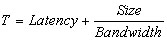
Point to point communications are modeled using the parameters latency and bandwidth, thus the time for a message for being delivered is computed as:
Collective communication
Global communications model use a different formula to compute the duration of the message, and synchronization is included before the communication itself. Although not all implementations of global operations require synchronization, good results suggest us to maintain this simple model. Figure 5 shows the timing model for collective communication.
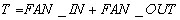
Many collective operations have two phases: a first one, where some information is collected (fan in) and a second one, where the result is distributed (fan out). Thus, for each collective operation, communication time can be evaluated as:
FAN_IN time is calculated as follows:
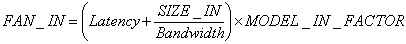
Depending on the scalability model of the fan in phase, the parameter MODEL_IN_FACTOR can take the following values:
| MODEL_IN | MODEL_IN_FACTOR | |
|---|---|---|
| 0 | 0 | Non existent phase |
| CTE | 1 | Constant time phase |
| LIN | P | Linear time phase. P = number of processors |
| LOG | N steps | Logarithmic time phase |
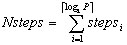
In case of a logarithmic model, MODEL_IN_FACTOR is evaluated as the Nsteps parameter. Nsteps is evaluated as follows: initially, to model a logarithmic behavior, we will have é log2 P ù phases. Also, the model wants to take into account network contention. In a tree-structured communication, several communications are performed in parallel in each phase. If there are more parallel communications than available buses, several steps will be required in the phase. For example, if in one phase 8 communications are going to take place and only 5 buses are available, we will need é 8/5 ù steps. In general we will need é C/B ù steps for each phase, being C the number of simultaneous communications in the phase and B the number of available buses. Thus, if stepsi is the number of steps needed in phase i, Nsteps can be evaluated as follows:
For FAN_OUT phases, the same formulas are applied, changing SIZE_IN by SIZE_OUT. SIZE_IN and SIZE_OUT can be:
| SIZE_IN | Description |
|---|---|
| MAX | Maximum of the message sizes sent/received by root |
| MIN | Minimum of the message sizes sent/received by root |
| MEAN | Average of the message sizes sent and received by root |
| 2*MAX | Twice the maximum of the message sizes sent/received by root |
| S+R | Sum of the size sent and received root |