Basic results
Dimemas results include global application information: execution time and speedup. For each task, computation time, blocking time, and information related to messages: number of sends, number of received (divided in number of receives that produces a block because a message is not local to the task, and number of messages that promotes no block).
Application analysis
Once the trace file has been obtained, what are the logical steps to follow? Here follows the typical steps, using the NPB LU benchmark, CLASS B using 8 processors, but only a single program iteration.
- Is my application well balanced? Are there any dependencies?
Executing the simulator with ideal network conditions, infinite bandwidth, zero latency and no bus contention. Dimemas reports a speedup of 7.55 over 8 processors. This corresponds to an average efficiency of 0.94. The output of Dimemas for each process shows that the individual efficiencies vary from 0.92 to 0.98. From this we can infer that overall the application is well balanced and that the performance loss due to precendences is not important. Of course, the numbers reported by Dimemas are global for the whole run. It is recommended to have a look at the Paraver trace that Dimemas can generate to get a better understanding on the behavior along time.
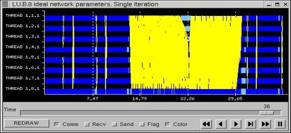
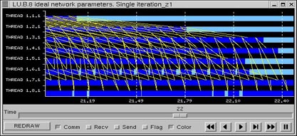
The LU execution time with these parameters setting is 36.97 seconds. Figure 29 is the view graph of the complete iteration of LU. Red areas refer to blocking time due messages are not ready to be received (as long as an ideal network has been used, the contention of the application is due to application implementation). Zooming to Figure 30, we can observe for process 0 a blocking time close to 2.5 seconds, but also process 5 is being block many times because message is not ready.
-
Can we improve the application grouping messages? Does latency influence application time?
Set up a group of experiments, using different latencies and an ideal bandwidth.
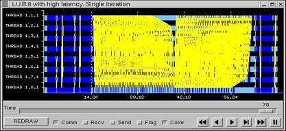
Results in Figure 31 show clearly that NPB LU application time is not having influence from message latency for typical values less than 1 ms. If we use an exagerated latency of 50 milliseconds, the result is presented in Figure 32. Compared to Figure 29 we observe an enormous influence of latency in some part of the trace (many small messages), while not relevant in other parts (few large messages).
- Are we planning to run our application in a low bandwidth network? Does bandwidth have influence in application time?
Using a fixed latency (ideal), the application time for different communication bandwidth is presented in Figure 33.
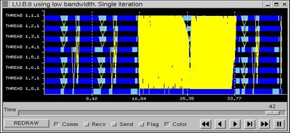
As reported by Dimemas (Figure 33), a bandwidth of 10MB/s is sufficient for this application. Comparison of Figure 34 (0.5 MB/s) and Figure 29 (instantaneous) shows the influence of bandwidth in the application. Big messages (located before and after the area with more communications) use a lot of time, and then parallelism of different tasks is reduced.
- Do resources limit application time?
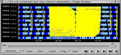
In the previous case we assumed that the network supported as many concurrent communications as needed by the application. What will happen if there were only one communication at a time as would happen in an Ethernet network of workstations? Comparison of Figure 29 and Figure 35 clearly shows the influence in this situation, large message produce important delays in other messages. The total execution time goes from 44.17 to 67.52 seconds because of the network contention.
Additional analysis
What if analysis
Can we improve the application time if some application function is optimized/vectorized? Is it important for the application to improve my network?
You can get solution to those questions using "What if analysis". The cost (time spent in a given function) can be reduced/enlarged specifying a ratio. Thus the execution time within the function the simulator will use, is that in the tracefile but modified with the factor.
Critical Path
This analysis provides information of those functions/subroutines in the application, rated based in the total computation/communication time spent in each function. This information is valuable in order to optimize the application (reduce the cost of the most computation time consuming) and to balance properly the application (reduce the most communication time, because this is mainly due to blocking time). In Figure 37a, rhs, erhs, ssor are the most important ones related to computation. MPI_send is in Critical Path 1% of execution time.
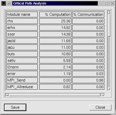
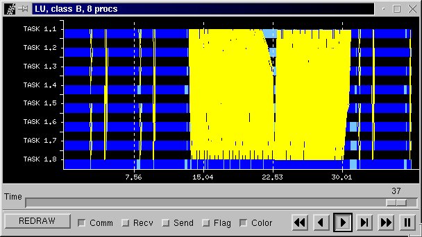
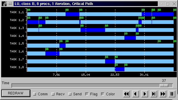
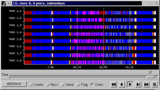
Figure 37b is the Paraver view of the application including all communications. The Critical Path is presented in Figure 37c. Figure 37d is visualization of the different subroutines called in the application. Each colour representd a different subroutine.
Synthetic Perturbation Analysis
The Synthetic Perturbation Analysis computes which are the most influent factors to application time, communication time, and computation time.
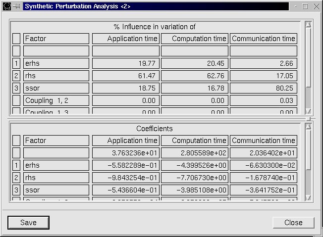

The analysis is performed using interpolation and factorial analysis. In the previous figure, three parameters analysis is performed, based in subroutines rhs, erhs and ssor. The most influent factor is rsh function, which explains close to 62% the variation of application time. This subroutine had the most important participation in the application critical path, but not in this magnitude.