Qualitative validation
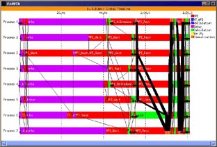
The qualitative usefulness of Dimemas can be perceived by looking at Figures 6, 7 and 8. Figure 6 displays the Vampir visualization of the LU benchmark (Workstation class) in a dedicated environment (only two iterations are shown in order to reduce the trace file size). The application was run on an SGI O2000 and traces with absolute times were generated by VAMPIRTrace. The total execution time is 1.7 seconds.
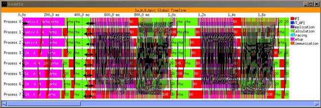
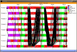
Figure 7 corresponds to the same application but the traces obtained in a heavily loaded system. Each image corresponds to a different execution of the application. As can be seen, the application behavior differs in each execution. The execution time of each run is 80, 26, 24 and 53 seconds respectively.
|
|
|
 |
 |
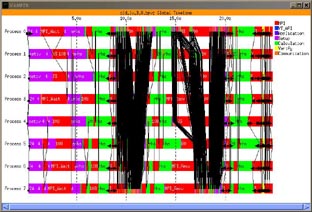
The four runs had totally different elapsed times and although the communication pattern are certainly the same, it is not possible to draw conclusions about what is the performance limiting factor or where should tuning effort be concentrated.
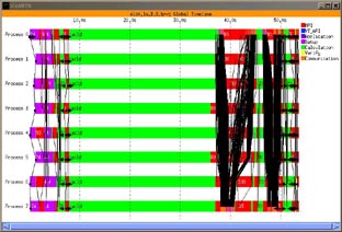
Figure 8 corresponds to the same program and number of iterations, but the visualization tracefile has been obtained with Dimemas. Dimemas tracefiles have been obtained in the same highly loaded environment and then running Dimemas with a latency of 28 microseconds and bandwidth of 82 MB/s (values reported by a Ping-Pong benchmark).
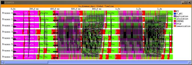
Comparing Figures 6 and 8 we can conclude that the behavior of the application is similar, allowing the utilization of Dimemas tracefile to predict the behavior of the application not using a dedicated machine. As can be seen, the similarity with the current parallel run is good. The Vampir trace generated in this way can be used to analyze the application and identify possible optimizations. We could like to state other type of qualitative validation coming from an end user statement: “I can identify better the structure of my application on the Dimemas generated Vampir trace than on a real Vampir trace”
Stability
The question may arise of what would happen if we repeat the tracing and Dimemas process. Are the results stable enough? Will we the huge variation observed with Vampir appear again?
It is certainly true that several instrumented runs will generate different Dimemas traces. Memory related issues are the major source of variation. Cache pollution generated by the multiprogramming OS scheduling policies will have the major effect, but also data placement issues and process migrations will be important in a NUMA machine.
To evaluate this effect we carried out an experiment where 30 runs of a benchmark (NAS LU on 32 processors) were run on a loaded machine. For each of them, a Dimemas trace was generated and the elapsed time measured. In the following figure we plot the current elapsed time (in seconds) of the instrumented run versus the time Dimemas predicts it would have taken if run on 32 dedicated processors.
As can be seen in Figure 9, there is a correlation between the current elapsed time and the predicted time, showing that the runs that experienced more delay also introduced more perturbation in the trace due to cache problems. The variability of the predicted time is nevertheless minimal compared to the variations in elapsed time (4% vs. 210%)
Figures 10 shows a similar experiment (LU) with 16 and 8 processors. In the 16 processors case, the variability of predicted time is below 2%. The variability of elapsed time is above 20%. As can be seen the more processors are used, the more predicted and elapsed time variance is, but the variance for the predicted time is kept within a reasonable value for this benchmark. The same conclusions are valid for the 8 processors case.
 |
 |
Will other codes behave the same?
We repeated the same type of experiment with other benchmarks. Figure 11 corresponds to the Barrier benchmark. The results show that the predicted range spans a variation of 39% while the variation of the elapsed time is 452% (256% without the outlier). Even if we eliminate the outlier taking more than 60 seconds, the variation of the real run is much higher that that of the predicted time. The variance of the prediction is nevertheless much higher that in the previous case (LU). This has to be attributed to the fact that the Barrier benchmark does not carry out any useful computation between successive MPI calls. The CPU burst that the Dimemas tracing generates are thus very small, and a minimal error in the clock precision reflects directly on the total predicted time.
We also performed 25 samples of the SP benchmark with 16 processors. The elapsed time variability is 73% and the predicted time variability is 16%. SP is a benchmark with very small CPU bursts between communications. This is reflected in larger variability than the LU benchmark. We nevertheless consider that 16% is quite acceptable. Our claim is that the quality and stability of results makes of Dimemas and adequate methodological tool for performance analysis of message passing programs.
Parameter optimization for micro-benchmarks
In order to evaluate the quality of the predictions we performed an optimization process for different micro-benchmarks that intensively stress some of the communication primitives in MPI. Each of them was run with dedicated resources, a Vampir trace with dedicated resources was also obtained and then a Dimemas trace was obtained in a loaded system. Then, for each of the benchmarks a whole bunch of simulations was done trying to fit the elapsed time of the dedicated run by using the Dimemas trace and varying the latency and bandwidth parameters.
The following plots show the ranges of bandwidth (Figure 13)and latency (Figure 14) that lead to predicted time within 10 % of the dedicated elapsed time. On the X-axis, different benchmarks and collective models are presented. Table 3 contains the parameter setting for the collective communication model for SGI O2000.
| MPI Call | Fan in model | Fan in size | Fan out model | Fan out size |
|---|---|---|---|---|
| MPI_Barrier | Lineal | Max | 0 | |
| MPI_Bcast | Log | Max | 0 | |
| MPI_Gather | Log | Mean | 0 | |
| MPI_Gatherv | Log | Mean | 0 | |
| MPI_Scatter | 0 | Log | Mean | |
| MPI_Scatterv | 0 | Log | Mean | |
| MPI_Allgether | Log | Mean | Log | Mean |
| MPI_Allgatherv | Log | Mean | Log | Mean |
| MPI_Alltoall | Log | Mean | Log | Max |
| MPI_Alltoallv | Log | Mean | Log | Max |
| MPI_Reduce | Log | 2Max | 0 | |
| MPI_Allreduce | Log | 2Max | Log | Max |
| MPI_Reduce_Scatter | Log | 2Max | Lineal | Min |
| MPI_Scan | Log | Max | Log | Max |

Our conclusion is that the proposed model is simple enough to capture acceptably well the performance of communication primitives.
Quantitative validation
We have selected the benchmarks BT, CG, FFT, IS, LU, MG and SP, with the classes W and A. The number of tasks for the experimentation is 8, 16 and 32 for CG, FFT, IS, LU and MG; and 9, 16 and 25 for BT and SP (because both benchmarks require a exact square root number of tasks). The parameters we will use for this validation are:
- Latency = 25 mseconds
- Bandwidth =87.5 Mbytes/seconds
- 1 half-duplex link
- 16 buses
- Collective operation model: refer to Table 3
Figure 15 presents the predicted time versus the real execution time. Each point represents a different experiment (benchmark, class, tasks). The lineal model fits very well with this data representation, showing that prediction and measuring data are very close. The problem in this representation is that most benchmarks results are located in the same area, close to origins.
Figure 16 presents the same results but with a different graphic. In the X-axis, we present the 42 different benchmarks. Dedicated is the application time in a dedicated environment. Instrumented is the application time for the same application but tracing the execution. And, finally, prediction is the predicted time for the application. The accuracy seems to be adequate once again, because once again some benchmarks are having a big execution time, and have a lot of influence in the graphical representation.
Figure 17 presents the same results are presented as error. Most of the benchmarks are predicted with less than a 10% of error. The point out of the graphic takes the value 150% error. This error and those over 10% refer to really short executions (less than five seconds). Thus the real difference between execution and prediction is negligible.